Classification of optical coherence tomography images using deep machine-learning methods

Full Text

BACKGROUND

Optical coherence tomography (OCT) is a modern, high-tech, conclusive method for detecting retinal and preretinal vitreous abnormalities [1]. However, describing and interpreting the examination results requires highly skilled and trained HCPs and a considerable duration on the part of ophthalmologists and patients. Therefore, we must solve issues associated with the automation of OCT image classification.

Computerized tools and technologies are rapidly evolving to build artificial intelligence (AI) systems based on neural networks with various architectures, for medical [2, 3] and general use [4–6]. In the past decades, advanced ophthalmology centers have created repositories of patient data with hundreds of thousands of OCT images, paving the pathway to (i) search for generalized dependencies and relationships between individual parameters and (ii) construct fundamentally new, science-based approaches for identification, classification, calculation, and prediction, all of which are almost always centered on a mathematical model.

In one of our papers, we have already described computerized methods for the examination of the vitreous body, identification and approximation of the retinal border, determination of its curvature, calculation of average retinal thickness, among others; one of these methods include artificial neural networks (ANNs) [7]. This study is a logical continuation of that research and presents results of OCT image classification achieved via convolutional neural networks (CNNs) using single- and multi-model approaches.

There have been many publications on similar topics. For example, Yu. A. Vasiliev et al. [8] developed a general, AI-based methodology for software testing and monitoring in medical diagnostics. The methodology enhanced the quality of this software and implementation in clinical practice. It consisted of seven steps: self-testing, functional testing, calibration testing, process monitoring, clinical monitoring, feedback, and improvement. The methodology was characterized by the cyclical phases of testing, monitoring, and improving the software for continuous improvement of software quality, detailed requirements for outcomes, and involvement of HCPs in software evaluation. The methodology allowed software developers to achieve remarkable results in various areas and enabled users to make informed and confident choices from programs that passed an independent and comprehensive quality check.

Katalevskaya et al. [9] developed algorithms for segmentation of visual signs of diabetic retinopathy and diabetic macular edema in digital fundus images acquired using a fundus camera. Features included in the International Classification were selected for segmentation: microaneurysms, hard exudates, soft exudates, intraretinal hemorrhages, retinal and optic disc neovascularization, preretinal hemorrhages, epiretinal membranes, and laser coagulates. Neural networks were implemented and trained using the deep-learning framework TensorFlow (Google Brain, USA). The training database contained 1,200 images, and 310 fundus images were used for validation. The accuracy of identifying these features by the trained model ranged from 86% to 96%.

T. Kerr et al. [10] described a home monitoring system for age-related macular degeneration. CNNs were used to segment the entire retina and pigment epithelial detachments. The dataset of 711 images was divided into training/validation/test image sets in the ratio of 60%:20%:20%. The CNN-based approach reportedly provided accurate retinal segmentation.

Sakhnov et al. [11] developed a cataract screening model based on an open dataset to validate the model based on clinical data. The open dataset comprised 9,668 images acquired using a smartphone camera, of which 4,514 were for “cataract” eyes and 5,154 for “healthy” eyes. The external validation set included 51 cataract and normal images. A machine learning model was built using CNN. The accuracy of data classification was 97% for the internal validation set and 75% for the external validation set. These authors noted predictive value to be low and concluded that they needed to refine their model to meet the performance metrics.

Shukhaev et al. [12] employed the pretrained networks ResNet-18, ResNet-50, VGG16, VGG19, and GoogleNet to solve the problem of using CNNs for automatic detection of Fuchs’ dystrophy. A random sample (n = 700) of corneal biomicroscopic images was obtained using a Tomey EM-3000 endothelial microscope (Tomey Corporation, Japan). In the first step, the images were categorized into two groups: the first group included images showing Fuchs’ dystrophy, whereas the other one included normal images or images of other abnormalities. The images of the endothelial cell density were arranged into three categories: training, validation, and test datasets. The following F-metric values were obtained while testing the neural network on a test sample for various CNN architectures: ResNet-18, 0.985; ResNet-50, 1.000; VGG16, 0.940; VGG19, 0.990; and GoogleNet, 0.987. ResNet-50 demonstrated the optimum performance with ImageNet data that had frozen layers, Adam optimization algorithm, and cross-entropy as the loss function.

Therefore, a brief analysis of the abovementioned studies allowed us to conclude the prospects of use of CNN-based ANN models for retinal OCT image classification.

AIMS

Our objectives were:

1. to develop architectures of mathematical (computerized) models based on deep-learning CNN for classifying OCT images using the libraries Python Keras and TensorFlow in Google Colaboratory,
2. to compare the results of computational experiments to classify OCT images obtained using single- and multi-model approaches and to evaluate the accuracy of such classifications, and
3. to conclude on the optimal architecture of ANN models regarding classification accuracy and the hyperparameter values used.

MATERIALS AND METHODS

The initial dataset comprised anonymized OCT images of real patients and included 1,004 images directly obtained as JPG files from the DRI-OCT Triton tomograph (Topcon Corporation, Japan) at a resolution of 1,920 × 969 × 24 BPP. For classification purposes, the entire dataset was categorized into the following 12 classes by experienced ophthalmologists:

1. Normal
2. Cystoid macular edema
3. Neuroepithelial detachment
4. Pigment epithelial detachment
5. Hard exudates
6. Epiretinal membranes
7. Vitreomacular adhesion
8. Posterior vitreous detachment
9. Full-thickness macular hole + epiretinal membrane
10. Hard exudates + cystoid macular edema
11. Pigment epithelial drusen
12. Lamellar macular hole + epiretinal membrane

The number of images in each class corresponded to the incidence of the corresponding abnormality in the patients. In subsequent computational experiments, new OCT images were added to the dataset, following which the total number of images exceeded 2,000. A fragment of 1,100 × 550 × 24 BPP was cropped from the entire subject area image to create the training, validation, and test datasets. In computational experiments, the entire data set was usually divided into training, validation, and test sets in the ratio of 70%:20%:10%.

The following technological methods were also used:

• Image rescaling using filters NEAREST, BILINEAR, BICUBIC, and LANCZOS
• Data augmentation via various options, such as image rotation by a given angle, shifting the image along the X and Y axes, horizontal and vertical rotation, and changing the brightness of the image channel

The optimum results in this study were obtained with the simplest NEAREST filter, which uses the parameters of nearest pixel. More complex filters that approximate the region using different methods gave poorer results, apparently because small image details important for classification were lost during the smoothing process.

The following parameters were used while compiling the model:

• Adam optimizer as one of the most effective optimization algorithms
• Categorical_crossentropy loss function
• Accuracy metric as percentage of correct answers given by the algorithm

The accuracy metric is usually used to solve classification problems when the number of images between the groups is balanced. Herein, we estimated an overall average because of the small number of images in the training and test sets. Python language tools were used in Google Colaboratory for all technological processes with the models.

RESULTS

Preliminary computational experiments

Herein, we evaluated the effectiveness of various approaches to OCT image classification (such as the possibility of employing pretrained networks and transfer learning), image rescaling and augmentation techniques, and combinations of ANN model hyperparameters (number of convolutional and fully connected layers, batch size, among others).

For pretrained neural networks based on MobileNetV2 and MobileNetV3, the accuracies were 95%–98%, 61%–80%, and 41%–59% on the training, validation, and test sets, respectively. The image was scaled to 224 × 224 pixels to fit MobileNet.

Moreover, the abilities of different pretrained neural networks to learn using the given dataset were compared with transfer learning. The validation results were 80%, 81%, 79%, and 80% for MobileNetV2, ResNet101V2, InceptionResNetV2, and NASNetLarge, respectively.

For multilayer CNNs with traditional architecture (several Conv2D convolutional layers, each with a MaxPooling2D subsampling function, transforming the data pools into a one-dimensional Flatten tensor and several fully connected Dense layers), the accuracy of 70%–100% was achieved on the training set with a reasonable selection of epoch number. Comparatively, in the validation set, this number was considerably lower and had a wider range (35%–94%). In both cases, the validation accuracy was higher than the training accuracy, which may be ascribed to considerable heterogeneity in the training and validation datasets. The test accuracy was even lower, ranging from 27% to 59%, which is obviously not a satisfactory result.

The following conclusions were drawn after the preliminary experiments:

• The training set was unbalanced and heterogeneous and required correction and supplementation with new images.
• Although transfer learning models showed slightly better classification results, these results were inappropriate for ophthalmology practice. In addition, there were not many opportunities for improvement because of the freezing of the first hidden layers.
• The hyperparameters and the classification approach must be optimized to achieve acceptable classification accuracy.

Computational experiments: a single-model approach

Based on the preliminary experiments, new OCT images were added to the dataset, after which the total number of images increased to >2,000. The experiments tested various architectures of multilayer sequential CNNs, such as Several Conv2D convolutional layers, each with a MaxPooling2D subsampling layer and a layer that transformed into a one-dimensional Flatten tensor, and two fully connected Dense layers, the latter featuring the Softmax neuron transfer function suitable for solving classification problems.

The maximum number of convolutional layers is seven for a normalized image resolution of 512 × 512 pixels. All images in the dataset were rescaled using the Rescale tool. We tested CNN structures with two–seven such layers (Table 1) with simultaneous selection of the size and number of filters in the layers. Training was performed (typically with epochs = 15, BATCH_SIZE = 50, optimizer = “Adam,” loss = “categorical_crossentropy,” and metric = [“accuracy”]) for all computational experiments, as well as for validation and additional testing with images not previously included in the dataset.

Acceptable training and validation accuracies were achieved for almost all ANN models, except for the two-layer model (Table 1). However, the additional testing accuracy first increased with increasing number of convolutional layers, reaching a maximum value of 85% for the six-layer model and decreasing for the seven-layer model. Notably, the models presented here are currently positioned solely as a decision support system for an ophthalmologist. Considering that the dataset contained a limited number of images of various abnormalities, we accepted the level of 85% as sufficient for images to be classified by an ophthalmologist with limited experience. We concluded that an optimal number of layers was required for accuracy, which in this case was 6. However, this value may later change because new data will be added to the dataset and models will be retrained.

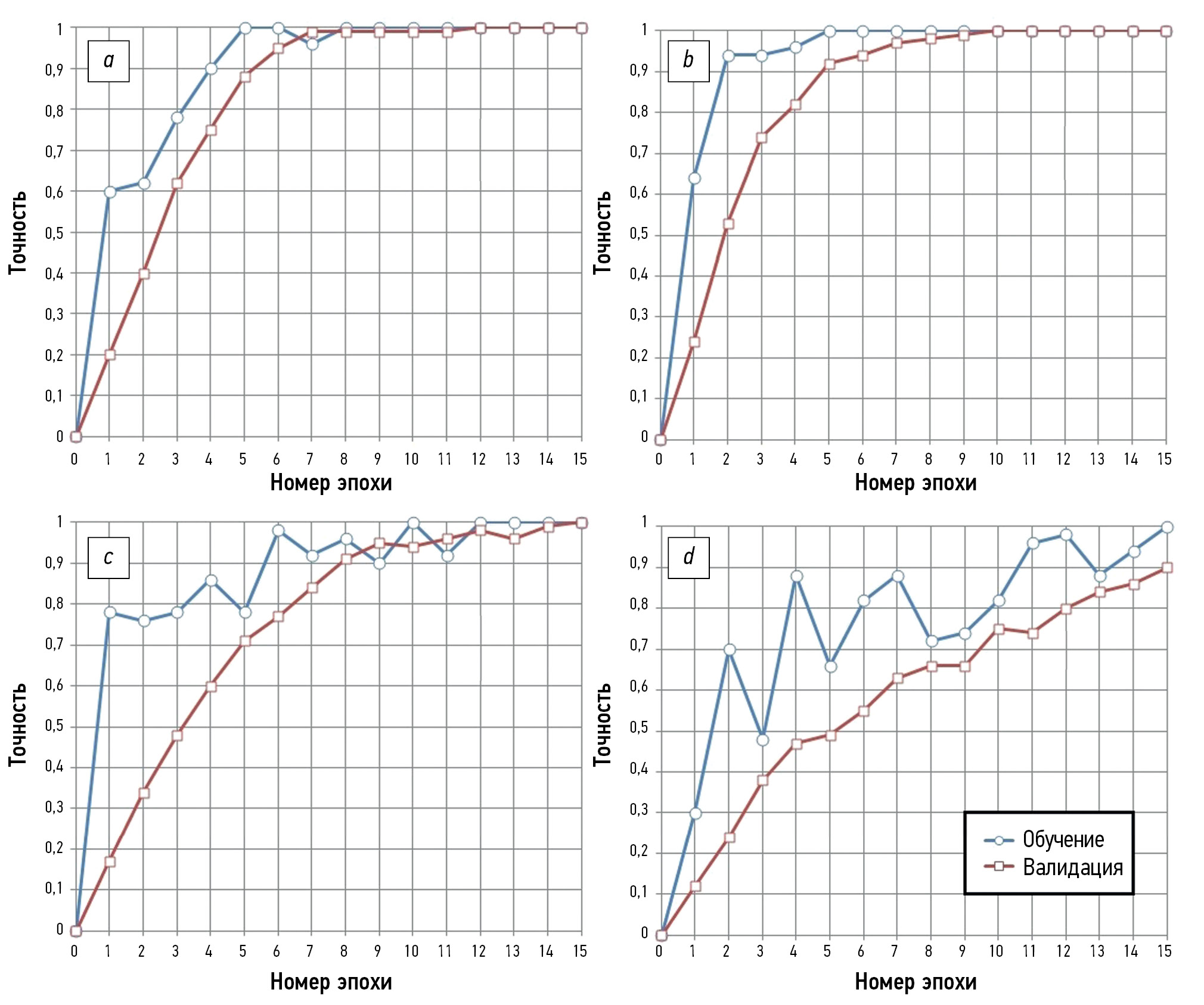
Fig. 1 shows the processes of ANN model training and validation with four to seven convolutional layers. The training process was completed in 9 epochs when four and five convolutional layers were used, achieving 100% training and validation accuracies. However, the accuracy of the additional test was only 65%–70% (Table 1). The training process was longer and consisted of 15 epochs when using a model with six convolutional layers, achieving 100% training and validation accuracies. However, accuracy in the additional test increased to 85%, which was considered satisfactory. Upon further increasing the number of convolutional layers to seven, the process for ANN model training and validating consisted of >15 epochs, while the training accuracy was 100%, and the validation and testing accuracies decreased to 89% and 74% (Fig. 1 and Table 1).

 

Fig. 1. Training and validation of convolutional neural network models with: a — four, b — five, c — six, and d — seven convolutional layers.

 

Table 1. Comparison of various sequential artificial neural network models

Number of convolutional layers	Number of parameters to be optimized	Training accuracy, %	Validation accuracy, %	Additional testing accuracy, %	Note
2	31 844 921	13	0	0	The ANN model is not trained well.
3	13 401 045	97	100	55	Number of ANN model training epochs: >15; number of filters in CNN layers: 3/8/16
3	15 215 889	100	100	62	Number of ANN model training epochs: 9; number of filters in CNN layers: 4/8/16
3	13 401 933	100	100	64	Number of ANN model training epochs: 12; number of filters in CNN layers: 5/8/16
4	6 929 729	100	100	65	Number of ANN model training epochs: 12
5	1 430 977	100	100	70	Number of ANN model training epochs: 9
6	556 673	100	100	85	Number of ANN model training epochs: 15
7	132 801	100	89	74	Number of ANN model training epochs: >15
8	–	–	–	–	8 CNN layers cannot be used for the accepted image size

Note. ANN, artificial neural network; CNN, convolutional neural network

 

Fig. 2 shows the architecture of the optimal ANN model concerning the accuracy of retinal OCT image classification. It includes six Conv2D convolutional layers with MaxPooling2D subsampling, a Flatten layer, and two fully connected Dense layers that act as classifiers, the latter featuring the Softmax neuron transfer function.

 

Fig. 2. Architecture and parameters of a six-layer convolutional artificial neural network model: the first number in Conv2D denotes the number of filters to be used in the convolution layer. The next two numbers represent the size (in pixels) of the filters. The activation functions of the network neurons are Relu and Softmax in the output classification layer. The first number in the fully connected Dense layer represents the number of neurons.

 

The lower classification accuracy in testing (compared with training and validation accuracies) is explained as follows: relatively small datasets of ~2,000 images were used to train the models, which did not contain a full set of graphical details characteristic of a particular abnormality. If such details are found in the test dataset, the classification may be deemed incorrect even when the ANN model validation accuracy is 100%.

Preliminary computational experiments: a multimodel approach

Following the general logic of the study and considering the need to increase the accuracy of additional testing, O. L. Fabrikantov and Ye.V. Kulagina proposed a sequential scheme that usually imitates the process of identifying a retinal OCT image by an ophthalmologist. Accordingly, a computer algorithm was developed (Fig. 3).

 

Fig. 3. Flowchart of a multimodel algorithm for optical coherence tomography image identification; ANN, artificial neural network; OCT, optical coherence tomography.

 

This algorithm is based on the sequential implementation of multiple models (Fig. 3). In Step 1, images were preprocessed (Blocks 1–3). In Block 4, ANN Model 1 was used, which was designed for a preliminary classification to distinguish between normal and abnormal images. The result of this classification was saved (S1). Such a model should be trained and validated on a special dataset 1 containing only two corresponding image classes. When no abnormality was detected (Block 5), we proceeded to Step 4 (examination of the vitreous body), bypassing all intermediate steps. As in Block 6, ANN model 2 was used, which is trained on a special dataset 2, to detect a macular hole. The result was saved (S2). If there was a macular hole (Block 7), then in Block 8, based on ANN model 3, also trained using a special dataset 3, we determined whether there was a full-thickness or lamellar macular hole. The results were saved (S3), after which we proceeded to Step 2.

If there was no macular hole (Block 7), we proceeded to Block 9, which used ANN model 4 trained on a special dataset 4 to detect one of the following three: cystoid macular edema, diffuse macular edema, or their absence. The result was saved (S4), after which we proceeded to Step 2.

Step 2 used ANN model 5 (Block 10) trained on a special dataset 5 to detect one of the following three: neuroepithelial detachment, pigment epithelial detachment, or their absence. The result was saved (S5), and we proceeded to Step 3 for the analysis and classification of OCT images.

In Step 3, ANN models 6, 7, and 8 were sequentially used.

• ANN model 6 (Block 11) was trained on a special dataset 6 to detect the presence or absence of epiretinal membranes.
• ANN model 7 (Block 12) was trained on a special dataset 7 to detect the presence or absence of drusen.
• ANN model 8 (Block 13) was trained on a special dataset 8 to detect the presence or absence of exudates.

The corresponding results were also saved (S6–S8) in Blocks 11–13, after which we proceeded to Step 4.

In Step 4, ANN model 9 (Block 14) was used, trained on a special dataset 9 to detect normal images, posterior vitreous detachment, vitreomacular adhesion, and vitreomacular traction, and the results were saved (S9). In Blocks 15 and 16, a general list of abnormalities was generated based on the previously saved S1–S9 data, and a report describing an OCT map was generated as a file.

DISCUSSION

In the described approach, nine different ANN models are used to classify abnormalities in OCT images, each model trained in its unique dataset (1–9). In the final step of examination of the vitreous body, the algorithm described earlier [7] can be used rather than the ANN model 9. It includes:

• vertical scanning of the image and determining the X and Y coordinates of the vitreous body borders,
• smoothing Y coordinates via the moving-average method with a base corresponding to minimum details of the image (10 pixels in our case), via approximation of the vitreous body border with a spline or parabola of the appropriate order, and
• calculating maximum border curvature and the corresponding distances to identify posterior vitreous detachment, vitreomacular adhesion, and vitreomacular traction.

Herein, a multimodel algorithm (Figure 3) was tested with an increasing number of OCT images in the datasets and optimized hyperparameters of ANN models. Preliminary computational experiments conducted for several steps of this algorithm indicated that 98%–100% accuracy can be achieved on training and validation sets with increased additional testing accuracy compared with the single-model approach, owing to the reduced number of factors classified at each step. Contextually, a single architecture with seven convolutional layers was used for all ANN models 1–9. The only difference is that they were trained on unique datasets and had different sets of coefficients of interneuronal synaptic junctions.

CONCLUSION

Single- and multi-model approaches were proposed for the classification of retinal OCT images. Computational experiments on automatic classification of such images obtained using a DRI-OCT Triton tomograph with various ANN model architectures indicated 100% accuracy on training and validation datasets and 85% for additional testing. This result is considered satisfactory. The ANN model with optimal architecture (6-layer CNN) was selected, and values of the corresponding hyperparameters were determined, further developing decision support systems for use in ophthalmology.

ADDITIONAL INFORMATION

Funding source. This study was not supported by any external sources of funding.

Competing interests. The authors declare that they have no competing interests.

Authors’ contribution. All authors made a substantial contribution to the conception of the work, acquisition, analysis, interpretation of data for the work, drafting and revising the work, final approval of the version to be published and agree to be accountable for all aspects of the work.

A.A. Arzamastsev — development of the concept, preliminary processing of OCT images, conducting research, writing programs, conducting computational experiments, multi-model approach to image classification, preparation of the manuscript; O.L. Fabrikantov — development of the concept, collection and preparation of OCT images, multi-stage classification scheme for OCT images, discussion and approval of the final version of the manuscript; E.V. Kulagina — development of a methodology for collecting and preparing OCT images, conducting research, a multi-stage classification scheme for OCT images, approval of the final version of the manuscript; N.A. Zenkova — concept development, research, editing and approval of the final version of the manuscript, analysis of literature data, editing the text of the article.

Acknowledgments. The work was carried out in accordance with the agreement on scientific and technical cooperation between Voronezh State University and the Federal State Autonomous Institution “National Medical Research Center” Interindustry Scientific and Technical Complex “Eye Microsurgery” named after Academician S.N. Fedorov””, Tambov branch dated November 28, 2022.

Master's degree students from the Faculty of Applied Mathematics, Informatics and Mechanics of Voronezh State University took part in the preliminary computational experiments: E.P. Galizina, V.A. Gushchina, I.O. Zavyalova, V.Yu. Kolupaev, N.M. Kushnarev, I.Yu. Novoskoltsev, E.A. Strukova, N.M. Chernyshov, I.D. Chikunov, A.A. Shcheglevatykh, as well as a diploma student M.A. Kuprin. These works were carried out under the guidance of one of the authors of the article.

About the authors

Alexander A. Arzamastsev

Voronezh State University; The S. Fyodorov Eye Microsurgery Federal State Institution

Email: arz_sci@mail.ru
ORCID iD: 0000-0001-6795-2370
SPIN-code: 4410-6340

Dr. Sci. (Engineering), Professor

Russian Federation, Voronezh; Tambov

Oleg L. Fabrikantov

The S. Fyodorov Eye Microsurgery Federal State Institution

Email: fabr-mntk@yandex.ru
ORCID iD: 0000-0003-0097-991X
SPIN-code: 9675-9696

MD, Dr. Sci. (Medicine), Professor

Russian Federation, Tambov

Elena V. Kulagina

The S. Fyodorov Eye Microsurgery Federal State Institution

Email: irina-kulagin2015@yandex.ru
ORCID iD: 0009-0006-0026-0832
SPIN-code: 8785-4949

MD

Russian Federation, Tambov

Natalia A. Zenkova

Derzhavin Tambov State University

Author for correspondence.
Email: natulin@mail.ru
ORCID iD: 0000-0002-2325-1924
SPIN-code: 2266-4168

Cand. Sci. (Psychology), Assistant Professor

Russian Federation, Tambov

References

Supplementary files