Оценка геометрических отклонений, возникающих при воспроизведении трёхмерных моделей средствами аддитивного производства, по данным компьютерной томографии

Полный текст

ОБОСНОВАНИЕ

Технология медицинского прототипирования, сочетающая в себе методы трёхмерного моделирования (computer-aided design, CAD) и трёхмерной печати, в последние десятилетия всё чаще используется в различных областях клинической и фундаментальной медицины [1–4]. Этому, в частности, способствует широкое распространение аддитивных установок, отмечаемое с 2000-х годов после запуска проекта самовоспроизводящихся 3D-принтеров (RepRap) и истечения срока патента на технологию печати методом послойного наплавления (fused deposition modeling, FDM).

Успешное применение медицинского прототипирования в клинической практике зависит от максимального соответствия получаемых изделий анатомии пациента [5]: в ряде случаев (печать персонализированных имплантатов, создание направляющих резекционных шаблонов) степень конгруэнтности напечатанного медицинского изделия и поверхности кости может непосредственно влиять на исход хирургического лечения [6]; в других ситуациях (предоперационная подготовка, создание тренировочных фантомов) точное воспроизведение геометрических соотношений между нормальными и патологически изменёнными тканями позволяет предвидеть возможные осложнения во время операции [7].

Препятствием для оценки точности получаемых моделей in vivo является сложность получения референтных значений размеров исследуемых анатомических структур. Прямое измерение объекта интереса не всегда осуществимо даже в процессе хирургического вмешательства (в связи с деформациями органов), а используемые для неинвазивного сбора морфологических характеристик органов методы медицинской визуализации сами лежат в основе получения трёхмерных моделей и их неточностей. В качестве альтернативы может быть использовано сравнение моделей, полученных на основе сканирования костных структур ex vivo, но при таком подходе используется относительно небольшое количество контрольных точек, а сложность их интерпретации различными специалистами может приводить к ошибкам [8]. Хорошие результаты с последующим их внедрением в клиническую практику дают испытания на 3D-моделях крупных млекопитающих (например, свиньях) [9].

В более ранних работах, посвящённых оценке точности воспроизведения моделей средствами аддитивного производства, в качестве объектов исследования были выбраны физические модели. Их измерение проводилось по нескольким контрольным точкам прямыми средствами ― линейкой, штангенциркулем, координатно-измерительной машиной [10–12]. В настоящем исследовании предлагается использовать принципиально иной подход к оценке геометрических отклонений, который заключается в сравнении всех точек полигональной сетки, получаемой на основе аддитивных технологий с эталоном, представляющим исходную трёхмерную модель. Для этого в качестве эталона используется модель сложной формы и заранее известных размеров, спроектированная средствами параметрического моделирования. Сравниваемый объект, в свою очередь, представляет собой виртуальную модель, образованную на основе эталона в результате основных этапов медицинского прототипирования (трёхмерной печати, сканирования и моделирования). Такой подход позволит одномоментно оценить отклонения по всей поверхности изделия, не прибегая к многочисленным линейным измерениям и снижая влияние человеческого фактора на процесс измерения.

Цель исследования ― оценить геометрические отклонения, возникающие при воспроизведении объектов, имитирующих костную ткань, средствами трёхмерного моделирования (на основе данных компьютерной томографии) и аддитивного производства.

МАТЕРИАЛЫ И МЕТОДЫ

Дизайн исследования представлен на рис. 1.

 

Рис. 1. Дизайн исследования.

КТ ― компьютерная томография.

 

В программе для параметрического моделирования FreeCAD¹ (FreeCAD Community, ФРГ) спроектировали твердотельную модель на основе кубоида размерами 20×20×12 мм (д×ш×в), содержащую пять сквозных параллельных каналов диаметром 1; 2; 3; 4 и 10 мм, на верхней грани которой создали два углубления и два возвышения в форме полусферы и конуса (имитирующих скруглённые и заострённые выемки и выступы на поверхности костей) высотой 4 мм (далее ― эталон 1). Диаметр каналов был выбран с целью имитации на одном изделии различных отверстий черепа человека, визуализируемых современными методами компьютерной томографии (КТ). Шаг в 1 мм для каналов меньшего диаметра и неровности заданной формы на поверхности изделия применялись с целью мануальной оценки качества на этапе печати модели. При помощи программного пакета Blender² (Blender Foundation, Нидерланды) проводили расчёт объёмов, а также была создана копия данного эталона, увеличенная в 2 раза по длине, ширине и высоте (далее ― эталон 2), с целью проверки влияния увеличения размеров на величину линейных отклонений.

Параметрические модели, сохранённые в формате STL (Standard Triangle Language), загрузили в программу Repetier Host ³ (Hot-World GmbH & Co. KG, ФРГ), где при помощи слайсера CuraEngine⁴⁴ (Ultimaker, Нидерланды) провели генерацию файла G-code для 3D-принтера со следующими параметрами печати: высота слоя 0,2 мм, толщина стенок 0,8 мм, заполнение 33% (выбрано эмпирически), скорость 50 мм/с, температура сопла 210°C, температура платформы 50°C, принудительный обдув модели, ретракт 5 мм, коэффициент подачи 100%. Печать проводили на 3D-принтере Ender-3 (Creality3D, КНР) с диаметром сопла 0,4 мм PLA-пластиком BFCopper (Best Filament, Россия), содержащим частицы меди для имитации рентгеновской плотности костной ткани (среднее значение рентгеновской плотности пластика при 100% заполнении составило +1762 HU, σ=172 HU).

Полученные изделия отсканировали с использованием 128-срезового компьютерного томографа Ingenuity CT (Philips, Нидерланды) на воздухе с ориентацией каналов перпендикулярно плоскости гентри. Напряжение рентгеновской трубки составило 120 кВ, ток 117 мА, толщина среза 0,625 мм, размер пикселей реконструированных срезов 0,43×0,43 мм.

Серии томографических изображений в формате DICOM загрузили в программу 3D Slicer⁵ (3D Slicer Community, США). На их основе создали STL-модели эталона 1: четыре ― методом автоматического выделения вокселей с пороговыми значениями +500 HU, 0 HU, -500 HU, -750 HU соответственно (инструмент Threshold Paint), одну ― методом ручного посрезового обведения вокселей (инструмент Paint). Также создали одну модель эталона 2 методом автоматического выделения вокселей со значениями более -500 HU. Значения порогов для эталона 1 подобрали эмпирически, исходя из значений рентгеновской плотности в наружном слое модели (толщиной около 0,9 мм), составляющих -1000...+500 HU (-1000 HU заменено на -750 HU для исключения из модели окружающего воздуха). Выбор заведомо низких параметров (-500 HU, -750 HU) был обусловлен наличием выраженных дефектов при использовании положительных значений порога сегментации. Значение порога плотности для эталона 2 выбрали случайным образом из использованных для эталона 1 порогов.

Полученные модели загрузили в программу Meshmixer ⁶ (Autodesk, США), где производили анализ и исправление ошибок полигонизации, удаление структур, не контактирующих с наружной оболочкой моделей, а также перестройку сетки модели с фиксированной длиной края полигона (инструмент Remesh-Target Edge Length) равной 0,25 мм. Внешний вид модели на каждом из перечисленных этапов представлен на рис. 2.

 

Рис. 2. Внешний вид модели эталона 1 после этапов: а ― параметрического моделирования; b ― 3D-печати; c ― КТ-сканирования (аксиальный срез, уровень окна +805 HU, ширина окна 3718 HU, большая плотность выступов обусловлена более тесной укладкой филамента в горизонтальной плоскости); d ― создания полигональной сетки на основе КТ-данных.

 

На заключительном этапе модели, полученные на основе КТ-данных, вместе с соответствующими им эталонами попарно загрузили в программу CloudCompare⁷ (CloudCompare Project, Франция), где на основе итеративного алгоритма ближайших точек (Iterative Closest Point, ICP) производился расчёт линейных отклонений итоговой CAD-модели. Расчёт проводился от каждой вершины полученной полигональной сетки по нормали к ближайшей поверхности эталона. Статистические расчёты проводили с использованием программы GNU PSPP⁸ (Free Software Foundation, США).

РЕЗУЛЬТАТЫ

Определение объёма моделей проводили для предварительной оценки направления искажения их формы. В частности, если объём перестроенной полигональной сетки оказывался меньше (больше) объёма эталонной CAD-модели, то ожидалось уменьшение (увеличение) линейных размеров анализируемой модели. В случае равенства объёмов следовало ожидать либо совпадения размеров, либо их компенсированного искажения. Объёмы эталонов и моделей, полученных различными способами сегментации, приведены в табл. 1.

 

Таблица 1. Объёмы виртуальных моделей

Наименование модели: размеры кубоида, мм (тип и порог сегментации)	Объём, мм3	Различие с эталоном, мм3
Эталон 1	3576	—
20×20×12 (авто +500)	3607	31 (0,9%)
20×20×12 (авто 0)	3901	325 (9,1%)
20×20×12 (авто -500)	4255	679 (19%)
20×20×12 (авто -750)	4480	904 (25,3%)
20×20×12 (ручн.)	4538	962 (26,9%)
Эталон 2	28 608	—
40×40×24 (авто -500)	31 140	2532 (8,9%)

 

Обработанные инструментом Remesh полигональные сетки обладают примерно равной плотностью распределения вершин полигонов на единицу поверхности. При сопоставлении моделей (совмещение вершин кубоидов) с эталонами результирующим набором данных являлось количество узлов полигональной сетки, удалённых от поверхности CAD-модели на определённое расстояние (мм) в наружном (положительные значения) или внутреннем (отрицательные значения) направлении. Пример совмещения модели и получаемой при этом гистограммы отклонения точек поверхности представлен на рис. 3.

Рис. 3. Совмещение полигональных сеток моделей (а) и гистограмма рассчитанных отклонений линейных размеров (b).

 

Дополнительный пик в области положительных значений обусловлен анизотропностью вокселей вдоль оси Z, а также несколько избыточным нанесением материала на боковых гранях кубоида.

Полученные значения искажений геометрических размеров для каждой модели сведены в табл. 2.

 

Таблица 2. Показатели линейных отклонений размеров моделей

Наименование модели	Минимальное значение, мм	Максимальное значение, мм	Среднее значение, мм	Станд. отклонение, мм	Интегральная сумма, мм
20×20×12 (авто +500)	-0,58	1,146	0,026	0,214	1904
20×20×12 (авто 0)	-0,533	1,019	0,141	0,223	9532
20×20×12 (авто -500)	-0,421	1,129	0,296	0,211	20 756
20×20×12 (авто -750)	-0,675	1,107	0,373	0,197	27 179
20×20×12 (ручн.)	-0,809	1,068	0,411	0,253	18 190
40×40×24 (авто -500)	-0,862	1,353	0,37	0,275	50 213

 

Количество измерений, выполненных программой, соответствовало количеству вершин полигональной сетки (порядка 100 тысяч), а распределение отклонений линейных размеров приближено к нормальному. На основании полученных значений программой была построена гауссиана (вещественная функция Гаусса), аргумент максимизации которой был использован в качестве среднего отклонения линейных размеров данной модели. Для построения гистограммы все посчитанные программой линейные отклонения были разбиты по своим значениям на интервалы равной ширины ― классы. Для каждой модели рассчитали значение интегральной суммы (Sum) показателей линейных отклонений моделей:

$\mathrm{Sum} = \sum _{\mathrm{i}}^{\mathrm{n}} = ({\mathrm{d}}_{\mathrm{i}} \times {\mathrm{q}}_{\mathrm{i}})$         (1)

где d_i ― минимальное значение линейного отклонения в i-м классе, q_i ― количество представителей в i-м классе, n ― общее количество классов.

Линейное нормирование по формуле (2) было применено для каждой из величин (интегральной суммы и изменения объёма) с целью приведения их к безразмерному виду.

$\widetilde{{\mathrm{\chi }}_{\mathrm{i}}}=\frac{{\mathrm{\chi }}_{\mathrm{i}} ={\mathrm{\chi }}_{\mathrm{i}}– {\mathrm{\chi }}_{\mathrm{i} \min } }{{\mathrm{\chi }}_{\mathrm{i} \max }-{\mathrm{\chi }}_{\mathrm{i} \min }}$                   (2)

Линейно нормированные значения интегральных сумм сравнивали с показателями изменения объёма у соответствующих моделей для проверки направления искажения формы (рис. 4).

 

Рис. 4. Линейные нормированные значения: красный цвет ― различия объёма моделей с эталоном, синий цвет ― различия интегральной суммы линейных отклонений.

 

Сравнение значений интегральных сумм линейных отклонений и относительных изменений объёма моделей с использованием коэффициента ранговой корреляции Спирмена показало высокую корреляцию между ними (ρ=0,83; t_эмп=5,27, p=0,05). Таким образом, изменение объёма воспроизведённой модели соответствует линейным отклонениям, измеренным используемыми программными средствами.

ОБСУЖДЕНИЕ

Процесс создания медицинского прототипа включает в себя 3 основных этапа: сбор данных (сканирование), обработка данных (создание виртуальной модели) и 3D-печать [13].

На первом этапе проводится лучевое исследование, позволяющее получить данные о трёхмерном строении области интереса с высоким пространственным разрешением (компьютерная или магнитно-резонансная томография, трёхмерное ультразвуковое сканирование), результаты которого сохраняются в виде дискретизированных изображений формата DICOM (Digital Imaging and Communication in Medicine). Изменение геометрии на данной стадии может быть обусловлено спецификой получения и обработки диагностической информации выбранным методом визуализации.

Второй этап предполагает проведение сегментации (выделение вокселей медицинских изображений, относящихся к создаваемой модели), преобразование сетки вокселей в полигональную сетку и редактирование полученной трёхмерной модели. Сегментация бывает трёх видов ― ручной (полностью выполняемой оператором), полуавтоматической (выполняемой компьютером с коррекцией оператором) и автоматической (полностью выполняемой компьютером) [14]. Автоматизированные способы выглядят более привлекательными благодаря меньшим трудозатратам, но из-за особенностей используемых при этом компьютерных алгоритмов геометрия конечного изделия может быть сильно искажена, а их точность требует отдельного изучения [15]. Именно поэтому на данной стадии необходимо участие специалиста со знанием анатомии (в частности, лучевой) для корректного выделения и редактирования объектов интереса. Благодаря такому подходу основной причиной искажения геометрии на данной стадии является человеческий фактор.

На третьем этапе производится трёхмерная печать полученной виртуальной модели. Для его успешной реализации производится предварительная подготовка (слайсинг) модели, а после печати, при необходимости, осуществляется постобработка модели (удаление поддержек, обработка поверхности). Вклад данной стадии в искажение геометрии конечного изделия зависит в первую очередь от типа используемого аддитивного оборудования.

Таким образом, для оценки геометрических искажений в процессе прототипирования необходимо выполнение всех трёх его основных этапов на некотором физическом фантоме с заранее известными линейными размерами и задаваемыми характерными элементами конструкции. Известно, что условия сканирования и настройки печати способны оказывать воздействие на точность получаемого изделия [10, 16], поэтому соответствующие параметры сохранялись на одинаковом уровне для всех производимых моделей.

Существует множество различных программных пакетов, позволяющих проводить сегментацию медицинских изображений. Использование программы 3D Slicer на этапе создания виртуальной модели из DICOM-данных было вызвано доступностью (распространяется как «открытое» программное обеспечение) и наличием большого числа дополнительных модулей и расширений, делающих её идеальным инструментом для предоперационного планирования [17].

Полученные результаты подтверждают описанный ранее эффект «гантели», согласно которому уменьшение порогового значения автоматической сегментации приводит к расширению контура получаемой модели [8]. Так, при снижении порога с +500 HU до -750 HU среднее значение смещения точек поверхности от эталона последовательно увеличивалось с 0,026 до 0,373 мм соответственно. При этом можно заметить, что данные искажения в большей степени зависят от способа сегментации, чем от размеров сканируемого объекта, т.к. при пропорциональном увеличении модели в 2 раза во всех измерениях среднее значение линейных отклонений оказалось выше на 24% в сравнении с аналогичным показателем для моделей исходного размера с тем же порогом и на 10% ниже, чем у моделей исходного размера, сегментированных вручную.

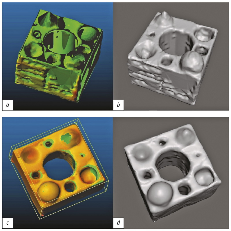
Относительно высокие значения геометрических отклонений у модели, сегментированной вручную (на 0,41 мм для образца с основанием 20×20 мм), могут быть вызваны выравниванием оператором боковых граней кубоида по рёбрам, которые оказались несколько смещены наружу (в процессе 3D-печати), что наблюдается также при сегментации полуавтоматическим способом. При этом стоит отметить, что данные модели лучше передавали исходную форму благодаря сохранению всех контрольных элементов и отсутствию дефектов стенок (рис. 5).

 

Рис. 5. Внешний вид моделей, сегментированных полуавтоматическим с порогом отсечения 0 HU (а ― с картой отклонений от эталона, b ― общий вид) и ручным (c ― с картой отклонений от эталона, d ― общий вид) способом.

 

При визуальной оценке моделей, автоматически сегментированных с порогом 0 HU и +500 HU, наблюдались дефекты стенки толщиной 1,2 мм, а у моделей с порогами -750 HU, -500 HU и 0 HU отсутствовали спроектированные сквозные отверстия диаметром 1 мм. Наличие дефектов, ширина которых превышает модуль минимальных отклонений геометрии, объясняется тем, что измерение толщины осуществляется по двум поверхностям, каждая из которых имеет отклонения (рис. 6).

Рис. 6. Измерение линейных отклонений от эталона (синие линии) в области дефекта сравниваемой модели (красные линии).

 

Таким образом, суммация линейного смещения вершины относительно внешней поверхности (отрезок d₁) со смещением близлежащей вершины относительно внутренней (отрезок d₂) может соответствовать дефекту стенки толщиной l, превышающему величину максимального линейного отклонения. Аналогично суммация положительных отклонений приводит к «заращению» отверстий, превышающих максимальное отклонение размеров, вычисленное по результатам работы алгоритма ICP. Именно поэтому при использовании полученных данных стоит иметь в виду, что линейные размеры воспроизводимых моделей включают в себя по два значения линейного смещения.

Каналы диаметром 1 мм, не выявленные на упомянутых экземплярах при визуальной оценке, также не были оценены алгоритмом, т.к. на моделях отсутствовали соответствующие данным каналам вершины полигонов.

Ограничения исследования

Ограничениями данного исследования могут являться относительно малый объём выборки, а также использование материала, не соответствующего истинному составу костной ткани.

ЗАКЛЮЧЕНИЕ

В процессе создания изделия средствами медицинского прототипирования (сканирование, 3D-моделирование, 3D-печать) неизбежно происходит искажение исходной формы. Изменение объёма моделей, как и средние линейные отклонения точек их поверхности от эталона, определённые при помощи итеративного алгоритма ближайших точек, имеют положительные значения. Искажение в большей степени зависит от выбранного способа сегментации, чем от общих масштабов модели или её частей. Использование ручного способа сегментации в сравнении с полуавтоматическим приводит к несколько большему искажению линейных размеров, вызванному выравниванием модели по недостоверным ориентирам, но позволяет воспроизводить все элементы исходного образца. Таким образом, в случае необходимости сохранения визуализируемых анатомических структур следует предусмотреть корректировку получаемых виртуальных моделей специалистом. При этом можно ограничиться использованием различных пороговых значений в зонах с плотными и разреженными структурами. Если же рядом мелких структур можно пренебречь, а основной задачей является соответствие общих габаритов изделия моделируемому органу, то предпочтительнее использовать полуавтоматическую сегментацию, порог которой должен быть подобран экспериментально в зависимости от тканевого состава и параметров сканирования.

ДОПОЛНИТЕЛЬНО

Источник финансирования. Авторы заявляют об отсутствии внешнего финансирования при проведении исследования и публикации статьи.

Конфликт интересов. Авторы декларируют отсутствие явных и потенциальных конфликтов интересов, связанных с публикацией настоящей статьи.

Вклад авторов. А.В. Ширшин ― поиск публикаций по теме, анализ литературы, разработка дизайна исследования, обработка полученных результатов, написание текста; И.С. Железняк ― определение основной направленности обзора, экспертная оценка обзора литературы, разработка дизайна исследования; В.Н. Малаховский ― экспертная оценка обзора литературы, систематизация и финальное редактирование обзора; С.В. Кушнарев ― поиск публикаций по теме, определение материалов исследования; Н.С. Горина ― анализ литературы, определение методов исследования. Все авторы подтверждают соответствие своего авторства международным критериям ICMJE (все авторы внесли существенный вклад в разработку концепции, подготовку статьи, прочли и одобрили финальную версию перед публикацией).

Funding source. The authors declare that there is no external funding for the exploration and analysis work.

Competing interests. The authors declare no obvious and potential conflicts of interest related to the publication of this article.

Author contribution. Aleksandr V. Shirshin — search for relevant publications, literature analysis, research design development, data processing, writing; Igor S. Zheleznyak — determination of the main focus of the review, expert evaluation of literature review, research design development; Vladimir N. Malakhovsky — expert evaluation of literature review, systematization and final editing of the review; Sergey V. Kushnarev — search for relevant publications, determination of research materials; Nataliya S. Gorina — literature analysis, determination of research methods. All authors made a substantial contribution to the conception of the work, acquisition, analysis, interpretation of data for the work, drafting and revising the work, final approval of the version to be published and agree to be accountable for all aspects of the work.

 

Об авторах

Александр Вадимович Ширшин

Военно-медицинская академия имени С.М. Кирова; Национальный исследовательский университет ИТМО

Автор, ответственный за переписку.
Email: asmdot@gmail.com
ORCID iD: 0000-0002-1494-9626
SPIN-код: 4412-0498
Россия, 194044, Санкт-Петербург, ул. Академика Лебедева, д. 6Ж; 197101, Санкт-Петербург, Кронверкский пр., 49

Игорь Сергеевич Железняк

Военно-медицинская академия имени С.М. Кирова

Email: igzh@bk.ru
ORCID iD: 0000-0001-7383-512X
SPIN-код: 1450-5053

доктор медицинских наук, доцент

Россия, 194044, Санкт-Петербург, ул. Академика Лебедева, д. 6Ж

Владимир Николаевич Малаховский

Военно-медицинская академия имени С.М. Кирова

Email: malakhovskyvova@gmail.com
ORCID iD: 0000-0002-0663-9345
SPIN-код: 2014-6335

доктор медицинских наук, профессор, ассистент кафедры

Россия, 194044, Санкт-Петербург, ул. Академика Лебедева, д. 6Ж

Сергей Владимирович Кушнарев

Военно-медицинская академия имени С.М. Кирова

Email: S.v.kushnarev@yandex.ru
ORCID iD: 0000-0003-2841-2990
SPIN-код: 5859-0480

кандидат медицинских наук

Россия, 194044, Санкт-Петербург, ул. Академика Лебедева, д. 6Ж

Наталья Сергеевна Горина

Военно-медицинская академия имени С.М. Кирова

Email: natali_bgmu@mail.ru
ORCID iD: 0000-0002-6220-8195
SPIN-код: 8175-6746
Россия, 194044, Санкт-Петербург, ул. Академика Лебедева, д. 6Ж

Список литературы

Дополнительные файлы