Machine-learning technology for predicting intraocular lens power: Diagnostic data generalization

Full Text

BACKGROUND

Implantation of recent intraocular lenses (IOLs) allows ophthalmologists to effectively solve the surgical rehabilitation problems of patients with cataracts. However, the degree of improvement in the patient’s visual function is directly dependent on the accuracy of the preoperative calculation of the optical IOL power. For this reason, in ophthalmology, different formulas are designed to calculate this indicator. The most famous formulas include SRK II, SRK/T, Hoffer-Q, Holladay II, Haigis, and Barrett [1–7]. All these work well for an “average patient”; however, they are not adequate at the boundaries of input variable ranges. They have other drawbacks such as the following: first, they do not consider the nonstationarity of objects and setup when new empirical data are entered, such as in localization; second, the amount of input factors being considered is clearly insufficient. These circumstances result in many local corrections to the above formulas and their constant adaptation [2, 8].

The outstanding Russian ophthalmologist S.N. Fedorov (1967) is the world’s leader in “designing” formulas for calculating the optical IOL power [1, 2]. The most commonly used formulas for calculating the optical IOL power in ophthalmic practice include SRK/T, SRK II, Hoffer-Q, Holladay II, Haigis, and Barrett [3–7]. Several formulas for calculating the optical IOL power appeared in the late 1970s and early 1980s, and they were either theoretical or regressive. Surgeons used to prefer regression formulas, and one of the most successful formulas was the SRK formula developed by J.A. Sanders, D.R. Retzlaff, and M.C. Kraff [3–5].

Currently, there is an unprecedented development of artificial intelligence systems based on artificial neural networks (ANNs), which, with deep learning using large volumes of empirical data, make it possible to build adequate models in nearly any subject area, including biology and medicine [9–12]. Over the past decades, modern ophthalmology centers have created patient data storage that includes tens and hundreds of thousands of digitized indicator records.

In this situation, the construction of an intelligent expert system has clearly become a radical method for solving the problem of preoperative IOL calculation, the core of which would be a mathematical model built using ANN models. Compared with known formulas, such models could be trained based on stored data, which would consider a significantly larger number of relevant input factors and the region-specific nature of patients. A step-by-step retraining of ANN models on newly received data from the storage, and, if necessary, the modification of its structure would ensure its adaptability and solve the problem of considering the nonstationarity of the objects and localization of the model.

The first stage in constructing such an intelligent expert system is to solve the fundamental problem of generalizability of empirical data on a large number of patients using ANN models, identify significant observed input factors, and compare the adequacy of such models with known formulas [1–7].

AIMS

Thus, this study aimed to study the possibility of generalizing a significant amount of empirical data on IOL calculation obtained in one of the ophthalmological centers in Russia as a result of treating patients using a unified ANN model subjected to deep learning, identify the most significant observed input factors that greatly affect the preoperative IOL calculation error, and compare calculation errors made by ANN models and known formulas.

Background error calculation for optical IOL power

Previously, we have compared errors in the use of some formulas based on a significant amount of empirical data provided in an impersonalized form by the Tambov branch of the IRTC “Eye Microsurgery” named after Academician S.N. Fedorov [13]. Initial data were obtained at the end of 2014. The initial number of records was 28,940. Each record contained the following parameters: anonymous patient number, date of surgery, brand and optical power of the implanted IOL, age, eye length, required optical IOL power to correct refractive error and astigmatism (sphere and cylinder), and additional information related to the position of the IOL in the eye. The number of processed records was 11,701, and 17,239 records were not processed for the following reasons: the lens parameters were unknown or data in the fields were incorrect.

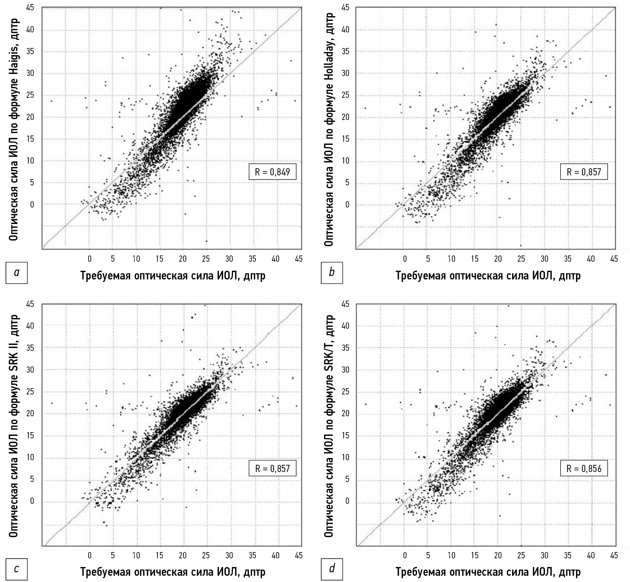
The Haigis, Holladay, SRK II, and SRK/T formulas were analyzed as being the closest to empirical data. The values of the mean relative errors in the IOL calculation are presented in Table 1. Fig. 1 shows the correlation dependence of the required and calculated optical IOL power according to these formulas. For the mean optical IOL power, all formulas give results close to the required ones; however, at extreme values, a significant scatter was observed with respect to the required values.

 

Table 1. Comparison of the IOL power calculation errors using different formulas

Formula	Mean relative error of the IOL calculation,%
Haigis	15.6
Holladay	13.4
SRK II	11.7
SRK/T	12.5

 

Fig. 1. Correlation dependence of the required optical IOL power along the horizontal axis and the calculated optical IOL power along the vertical axis according to the formulas: a) Haigis, b) Holladay, c) SRK II, and d) SRK/T for 11,701 patients. The correlation coefficients are shown in the graphs.

 

As shown in Fig. 1a, 1b, and 1d, a significant divergence is present in the slope angle of the dependence relative to the diagonal corresponding to the exact calculations. All the investigated formulas use three parameters as input values: eye length in mm (L), arithmetic mean of the meridians in mm (K), and anterior chamber depth as a lens parameter. This circumstance inevitably suggests the presence of other factors (possibly unobserved), and their effects on the optical IOL power led to the listed features of the calculation.

In the same study [13], we presented an optimized regression formula obtained by minimizing the mean square error for 11,701 patients using nonlinear programing methods. We managed to reduce the mean relative error to 10.6% by introducing a fourth variable. This means that additional input variables and ideally all relevant information about the patient should be considered. In this case, the ideal tool for predicting the optical IOL power is the use of ANN-based models.

A previous study by [14] is most related to our work. The study aimed to describe the use of machine learning in predicting the occurrence of postoperative refraction after cataract surgery and compare the accuracy of the model with formulas for calculating the optical IOL power. The training sample included data from 3331 eyes of 2010 patients. The model coefficients were optimized using data training. The occurrence of postoperative refraction was then predicted using conventional formulas: SRK/T, Haigis, Holladay 1, Hoffer-Q, and Barrett Universal II (BU-II). The absolute errors of some machine-learning methods were lower than those of the formulas. However, no statistically significant difference was found.

The results obtained in [14] appear to be quite expected because the authors did not use additional input parameters. The point is that machine learning and the least squares method, which are usually used for parametric identification of formulas, lead to comparable results. In the present study, we analyze the possibilities of using ANN models to predict the optical IOL power using a much larger number of input quantities.

The work on IOL calculations is sustained because of the need to reduce the IOL calculation error, emergence of data on new factors that were not considered in previous calculations (previously, only four input factors were considered compared with the current 26 input factors), desire to create an adaptive model for IOL calculation, which could consider possible nonstationarity of the incoming data, and the drive to create an expert system with dynamic knowledge acquisition and its step-by-step training based on ANN models.

MATERIALS AND METHODS

In 2021, ophthalmologist K.K. Syrykh provided initial data. They concern depersonalized results of both preoperative and postoperative observations of the patients. The original data file adopted for the construction of the ANN model included 455 entries: 26 columns of input factors (x₁–x₂₆) and one column for the output factor—IOL calculation (diopters), Y. The input variables were as follows: x₁, sex; x₂, visual acuity without correction before surgery; x₃, spherical component of refraction according to visometry data before surgery; x₄, cylindrical component of refraction according to visometry data before surgery; x₅, axis of the cylinder according to visometry data before surgery; x₆, visual acuity with correction before surgery; x₇, axis of the strong meridian of the cornea before surgery; x₈, refraction of the strong meridian of the cornea before surgery; x₉, axis of the weak meridian of the cornea before surgery; x₁₀, refraction of the weak meridian of the cornea before surgery; x₁₁, spherical component of the refraction according to refractometry data before surgery; x₁₂, cylindrical component of the refraction according to refractometry data before surgery; x₁₃, axis of the cylinder according to refractometry data before surgery; x₁₄, length of an eye (optical biometrics, mm); x₁₅, visual acuity without correction after surgery; x₁₆ spherical component of the refraction according to visometry data after surgery; x₁₇, cylindrical component of the refraction according to visometry data after surgery; x₁₈, axis of the cylinder according to visometry data after surgery; x₁₉, visual acuity with correction after surgery; x₂₀, axis of the strong meridian of the cornea after surgery; x₂₁, refraction of the strong meridian of the cornea after surgery; x₂₂, axis of the weak meridian of the cornea after surgery; x₂₃, refraction of the weak meridian of the cornea after surgery; x₂₄, spherical component of the refraction according to refractometry data after surgery; x₂₅, cylindrical component of the refraction according to refractometry data after surgery; and x₂₆, axis of the cylinder according to refractometry data after surgery.

For the convenient construction of ANN models, a simulator program previously developed by the authors was used [15].

RESULTS

One of the most complicated points in the development of ANN models is to propose a hypothesis about the structure (architecture) of the network.

The application of the theorems of A.N. Kolmogorov [16, 17] can often lead to an ANN model with a redundant structure. Generally, such a model suits well when representing the output variable at the nodal points; however, it has a weak predictive power.

In [18], we proposed a constructive algorithm that allows us to increase the number of neurons in the hidden layer and the number of hidden layers until certain conditions are reached. In this case, linear, quadratic, cubic, and other transfer functions of neurons are used rather than the commonly used sigmoidal transfer functions. Our approach is based on the expansion of the function of several variables in the Taylor series (1)–(2). Therefore, when expanding a function of many variables in a Taylor series, we must first introduce a differential operator:

${\mathit{T}}^{\mathit{k}}\mathbf{=}\mathbf{\sum }_{\mathbf{m}\mathbf{=}\mathbf{1}}^{\mathbf{n}}{\mathbf{(}{\mathbf{x}}^{\left(m\right)}\mathbf{-}{\mathbf{x}}_{\mathbf{0}}^{\left(m\right)}\mathbf{)}}^{\mathbf{k}}\frac{{\mathbf{\partial }}^{\mathbf{k}}}{\mathbf{\partial }{\mathbf{x}}_{\mathbf{k}}^{\left(m\right)}}$ (1)

The expansion of the function $f(x^{\left(1\right)},x^{\left(2\right)}, ... ,x^{\left(n\right)})$ in the Taylor series takes the following form:

$f\mathit{(}{x}^{\left(1\right)}\mathit{,}\mathit{ }{x}^{\left(2\right)}\mathit{,}\mathit{ }\mathit{.}\mathit{.}\mathit{.}\mathit{ }\mathit{,}\mathit{ }{x}^{\left(n\right)}\mathit{)}\mathit{ }=$

$=f\mathit{(}{x}_{\mathit{0}}^{\left(1\right)}\mathit{,}\mathit{ }{x}_{\mathit{0}}^{\left(2\right)}\mathit{,}\mathit{ }\mathit{.}\mathit{.}\mathit{.}\mathit{ }\mathit{,}\mathit{ }{x}_{\mathit{0}}^{\left(n\right)}\mathit{)}\mathit{ }+$                 (2)

$+\sum _k^p=1\frac{T^k(x^{\left(1\right)}, x^{\left(2\right)}, ... , x^{\left(n\right)})}{k!}+$

$+R_p(x^{\left(1\right)}, x^{\left(2\right)}, ... , x^{\left(n\right)})$

This makes it possible to obtain neural networks with a relatively simple architecture and good approximating (generalizing) and predictive abilities.

The ANN model, built in accordance with formulas (1) and (2), has a layer of input neurons, a functional hidden layer corresponding to several members of the Taylor series, a summing hidden layer, and an output layer. The functional hidden layer contains neurons with transfer functions corresponding to the terms of the Taylor series: linear (first order), quadratic (second order), and cubic (third order). The summing hidden layer contains one linear neuron, and its main function is to calculate the sum of several terms of a series and add a constant value to them. This architecture made it possible to achieve an acceptable accuracy of the ANN model.

The sum of the squared deviations of the model and empirical values was used as the loss function.

When training models based on empirical data, the following optimization methods were chosen: stochastic gradient method, simple gradient method, and gradient-free Gauss–Seidel and Monte Carlo coordinate descent methods, which were used interactively.

The starting point for training the ANN model based on the IOL data was a network consisting of 26 input neurons, one linear neuron in the hidden layer, and one output neuron. Such a construction corresponded to the free and first terms in formulas (1) and (2). Considering the recommendations of previous studies [8–11], the learning process of the model was carried out on 70% of the entire sample, whereas the predictive ability of the ANN model was assessed using the remaining 30% of the sample. Data for training and checking the adequacy of the model were selected from the general table at random using a uniform distribution of random variables.

The results of the training of this simple model are shown in Fig. 2. The true optical power of a given type of IOL to obtain emmetropia in each case was determined as the sum of the optical power of the implanted IOL and the resulting refractive error. The refractive error was calculated by retrospective analysis during the period from 1 to 6 months after surgery.

 

Fig. 2. Correlation of the calculated (Y_mod) and empirical data (Y_tab) for the first-order ANN model. The pair correlation coefficient is 0.84, and the mean relative error is 11.9%.

 

In terms of the mean relative error, they are comparable with classical formulas; however, in contrast, a linear function of 26 variables is used to predict the optical IOL power. Moreover, the pair correlation coefficient of the calculated and empirical data was 0.71, and the mean relative error was 11.9%.

The coefficients of synaptic connections for the channels of the linear model represent the sensitivity of the channels, and their values can be used to assess their degree of influence on the output variable. The numerical experiments showed that at least 12–15 input factors (available to the ophthalmologist) significantly affect the preoperative calculation of the optical IOL power. Consequently, our assumptions regarding the need to consider a larger number of input quantities to reduce the calculation error were fully confirmed. Significant errors in classical formulas [3–7] can be associated with the presence of a substantial number of input factors that are unobserved in these formulas.

Among the significant factors, the values of some factors (x₁₆, x₂₁, x₂₃, and x₂₄) become known only after surgery. However, these factors correlate well with similar factors, and their values can be obtained before surgery and are therefore well predictable.

Following our algorithm [18], we modified the structure of the ANN model so that along with the linear neuron in the hidden layer, a quadratic neuron was also present. The training of such an ANN model using similar numerical methods of nonlinear programing made it possible to reduce the mean relative error to 5%; thus, previous results were immediately improved by a factor of two. In addition, the pair correlation coefficient increased to 0.97, and the mean relative error was 4.8% (Fig. 3).

 

Fig. 3. Correlation of the calculated (Y_mod) and empirical data (Y_tab) for the second-order ANN model. The pair correlation coefficient is 0.99, and the mean relative error is 4.8%.

 

Following this logic, we also built a third-order ANN model containing neurons with linear, quadratic, and cubic transfer functions in the hidden layer. Training the ANN model by similar numerical methods of nonlinear programing made it possible to reduce the mean relative error up to 3.5%, with a pair correlation coefficient of 0.98 (Fig. 4).

 

Fig. 4. Correlation of the calculated (Y_mod) and empirical data (Y_tab) for the third-order ANN model. The pair correlation coefficient is 0.99, and the mean relative error is 3.5%.

 

The number of degrees of freedom of this ANN model equal to the number of synaptic connections 26 × 3 + 3 = 81 is significantly less than the number of entries in the training set. This circumstance confirms the good generalizability of empirical data on the calculation of the optical IOL power using the third-order ANN model.

Table 2 shows a comparison of various methods for calculating the optical IOL power. Therefore, when using ANN models and a significantly larger number of input variables, the mean relative error of calculations could be reduced by more than two times compared with using traditional methods.

 

Table 2. Comparison of the mean relative calculation errors of the optical IOL power and correlation coefficients of the calculated and empirical data for different methods

Formula and ANN model	Mean relative error, %	Correlation coefficient of the calculated and empirical data
Haigis formula	15,6	0,85
Holladay formula	13,4	0,86
SRK II formula	11,7	0,86
SRK/T formula	12,5	0,86
Linear ANN model	11,9	0,84
Nonlinear second-order ANN model	4,8	0,98
Nonlinear third-order ANN model	3,5	0,99

 

DISCUSSION

The next stage of research should be the collection of a significantly larger amount of data about patients because deep machine-learning methods require significant training samples. Then, the models should be validated on test samples [8–11]. If the system also contains hyperparameters, i.e., the parameters that must be set “from above” and the successful setting of which significantly affects the solution of the problem, then there must also be a third, additional test data sample. The availability of such data will make it possible to build an intelligent expert system for the preoperative calculation of IOLs, some of which are presented in our paper [19].

CONCLUSION

This study has the following findings: (1) The fundamental possibility of generalizing a significant amount of empirical data on calculating the optical IOL power using training ANN models that have a significantly larger number of input variables than when using traditional formulas and methods. The identification of the most significant observed factors that have a significant effect on the target indicator and their inclusion in the ANN model allows the reduction of the calculation error by more than two times. (2) The ability of ANN-based models to generalize data opens up the possibility of creating an intelligent expert system with a dynamic flow of new data and step-by-step deep machine learning of the intelligent core. The main feature of such a system, in comparison with the use of traditional calculation formulas, should be its adaptability, which allows solving the problems of the nonstationarity of an object and localization because of the presence of feedback in it. 3) Currently, the developed ANN model is used in conjunction with other calculation tools to preoperatively determine the optical IOL power in the mode of an ophthalmologist assistant.

ADDITIONAL INFO

Funding source. This study was not supported by any external sources of funding.

Competing interests. The authors declare that they have no competing interests.

Authors’ contribution. All authors made a substantial contribution to the conception of the work, acquisition, analysis, interpretation of data for the work, drafting and revising the work, final approval of the version to be published and agree to be accountable for all aspects of the work.

A.A. Arzamastsev — research concept, data processing, writing the manuscript, editing the manuscript; O.L. Fabrikantov — research concept, literature analysis, editing the manuscript; N.A. Zenkova — data processing, literature analysis, editing the manuscript; S.V. Belikov — preparing the dataset, searching for publications.

About the authors

Alexander А. Arzamastsev

Voronezh State University; The S. Fyodorov Eye Microsurgery Federal State Institution

Email: arz_sci@mail.ru
ORCID iD: 0000-0001-6795-2370
SPIN-code: 4410-6340

Dr. Sci. (Engineering), Professor

Russian Federation, Voronezh; Tambov

Oleg L. Fabrikantov

The S. Fyodorov Eye Microsurgery Federal State Institution

Email: fabr-mntk@yandex.ru
ORCID iD: 0000-0003-0097-991X
SPIN-code: 9675-9696

MD, Dr. Sci. (Medicine), Professor

Russian Federation, Tambov

Natalia А. Zenkova

Derzhavin Tambov State University

Email: natulin@mail.ru
ORCID iD: 0000-0002-2325-1924
SPIN-code: 2266-4168

Cand. Sci. (Psychology), Assistant Professor

Russian Federation, Tambov

Sergey V. Belikov

The S. Fyodorov Eye Microsurgery Federal State Institution

Author for correspondence.
Email: pvt.leopold@gmail.com
ORCID iD: 0000-0002-4254-3906
SPIN-code: 5553-8398

MD

Russian Federation, Tambov

References

Supplementary files